There are six types of algorithm that underpin the majority of ML models. In this section, we’ll focus on an overview of the algorithms, before exploring them in greater detail in the final two weeks of the module.
Some of this is revision of concepts and techniques we have covered earlier in the module.
73.2 Linear Regression
Theory
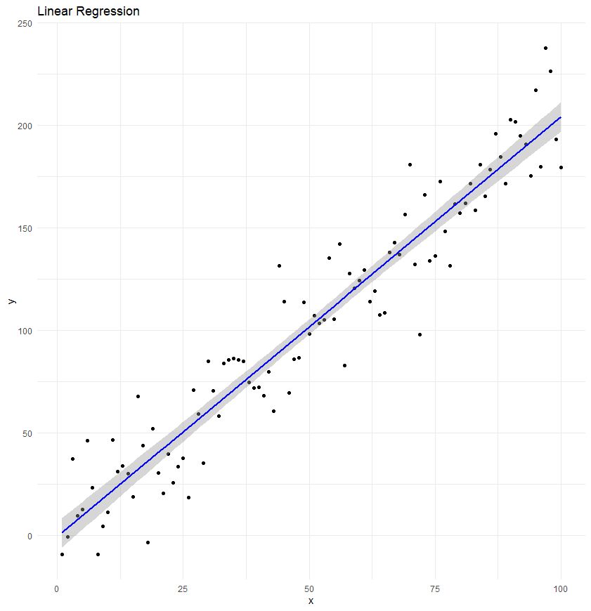
Linear regression is a statistical method used to model and analyse the relationship between a dependent variable and one or more independent variables.
The goal is to find a linear equation that best predicts the dependent variable based on the values of the independent variables.
In its simplest form, linear regression results in a straight line (in two dimensions) or a plane (in three dimensions) that minimises the differences (residuals) between observed values and the values predicted by the linear model.
The coefficients of the linear equation quantify the impact of changes in the independent variables on the dependent variable, allowing for both prediction and interpretation. Linear regression is widely used due to its simplicity, interpretability, and basis in classical statistical theory.
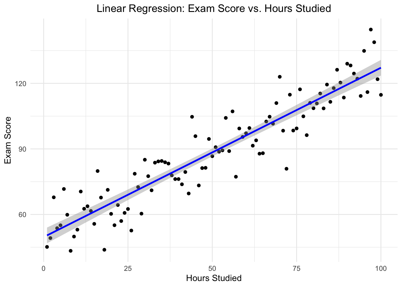
Example
# Set the seed for reproducibilityset.seed(123)# Generate a synthetic datasethours_studied <-1:100exam_score <-50+0.75* hours_studied +rnorm(100, mean =0, sd =10)# Combine into a data framestudy_data <-data.frame(hours_studied, exam_score)# Perform linear regressionmodel <-lm(exam_score ~ hours_studied, data = study_data)# Create a scatter plot of the data and the regression linelibrary(ggplot2)ggplot(study_data, aes(x = hours_studied, y = exam_score)) +geom_point() +# Plot the data pointsgeom_smooth(method ="lm", col ="blue") +theme_minimal() +labs(title ="Linear Regression: Exam Score vs. Hours Studied",x ="Hours Studied",y ="Exam Score") +theme(plot.title =element_text(hjust =0.5))
`geom_smooth()` using formula = 'y ~ x'
rm(model)
73.3 Logistic Regression
Theory
Logistic regression is used to model the probability of a certain class or event occuring, such as pass/fail, win/lose, alive/dead, or healthy/sick.
It’s used when the dependent variable is categorical and predicts the likelihood of the occurrence of an event by fitting data to a logistic function.
The outcome is binary or dichotomous, meaning there are only two possible classes.
Logistic regression estimates the parameters of a logistic model. It’s particularly useful for understanding the relationship between the binary response variable (DV) and one or more independent variables.
The coefficients from a logistic regression can be used to estimate odds ratios, providing insights into how each predictor is associated with the probability of the outcome.
This makes logistic regression a powerful tool for classification and prediction in various fields where it’s crucial to understand the factors that influence a binary outcome.
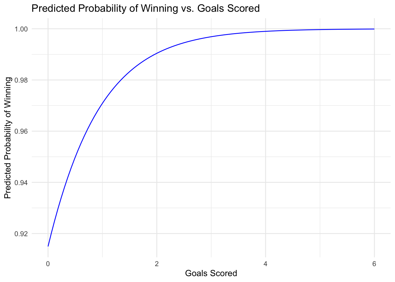
Example
set.seed(123)# Generate a synthetic datasetnum_matches <-100goals_scored <-rpois(num_matches, lambda =2)points_total <-rnorm(num_matches, mean =30, sd =10)# Create a binary outcome with association with goals_scored and points_total# Increase coefficients for the variables in the logistic functionwin_loss <-ifelse(runif(num_matches) <plogis(0.95* goals_scored +0.62* points_total -15), 1, 0)# Combine into a data framematch_data <-data.frame(goals_scored, points_total, win_loss)# Perform logistic regressionmodel <-glm(win_loss ~ goals_scored + points_total, data = match_data, family ="binomial")# Summary of the logistic regression modelsummary(model)
Call:
glm(formula = win_loss ~ goals_scored + points_total, family = "binomial",
    data = match_data)

Coefficients:
             Estimate Std. Error z value Pr(>|z|)
(Intercept)  -11.8202     3.1943  -3.700 0.000215 ***
goals_scored   1.1314     0.4597   2.461 0.013858 *
points_total   0.4818     0.1238   3.893 9.89e-05 ***
---
Signif. codes:  0 '***' 0.001 '**' 0.01 '*' 0.05 '.' 0.1 ' ' 1

(Dispersion parameter for binomial family taken to be 1)

    Null deviance: 97.245  on 99  degrees of freedom
Residual deviance: 33.814  on 97  degrees of freedom
AIC: 39.814

Number of Fisher Scoring iterations: 8
# Visualisationlibrary(ggplot2)# Create a new data frame for predictionsgoals_range <-seq(min(goals_scored), max(goals_scored), length.out =100)points_avg <-mean(points_total)prediction_data <-expand.grid(goals_scored = goals_range, points_total = points_avg)# Add predictionsprediction_data$win_prob <-predict(model, newdata = prediction_data, type ="response")# Plottingggplot(prediction_data, aes(x = goals_scored, y = win_prob)) +geom_line(color ="blue") +labs(title ="Predicted Probability of Winning vs. Goals Scored",x ="Goals Scored",y ="Predicted Probability of Winning") +theme_minimal()
73.4 K-nearest neighbours
Theory
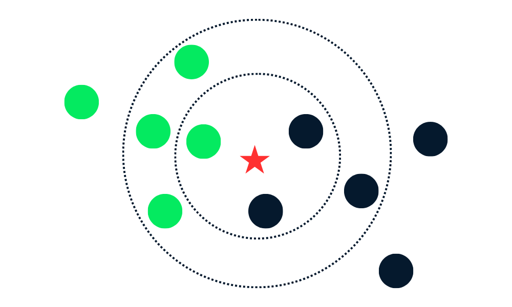
K-Nearest Neighbors (KNN) is a simple, yet powerful machine learning algorithm used for both classification and regression.
In the context of classification, KNN assigns a class to a data point based on the majority class of its ‘k’ nearest neighbors. It’s a type of instance-based learning, or “lazy learning”, where the function is only approximated locally, and all computation is deferred until function evaluation.
KNN is non-parametric, meaning it doesn’t make any assumptions about the underlying data distribution. This allows it to be used in a wide range of applications.
The key idea is that similar data points are near each other. Thus, by looking at the nearest neighbors of a point, we can classify it into a suitable category.
Example
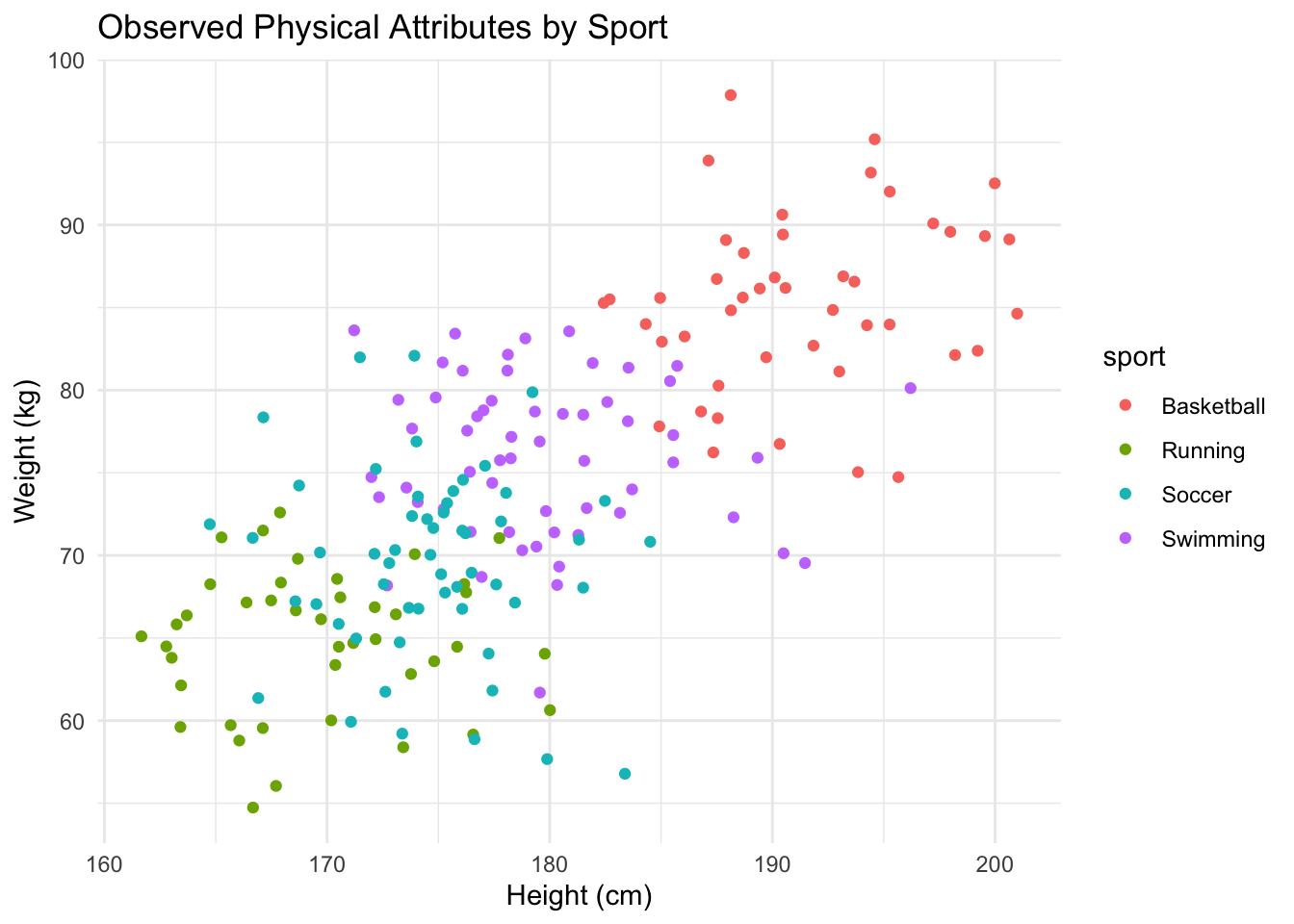
Our goal is to classify athletes into their respective sports using KNN, based on their physical attributes.
First, I’ll create a dataset and analyse the data visually.
# Load librarieslibrary(caret)
Loading required package: lattice
library(ggplot2)library(class)set.seed(123)# Generate syntheticnum_athletes <-200sport <-factor(sample(c('Basketball', 'Soccer', 'Swimming', 'Running'), num_athletes, replace =TRUE))height <-rnorm(num_athletes, mean =ifelse(sport =='Basketball', 190, ifelse(sport =='Soccer', 175, ifelse(sport =='Swimming', 180, 170))), sd =5)weight <-rnorm(num_athletes, mean =ifelse(sport =='Basketball', 85, ifelse(sport =='Soccer', 70, ifelse(sport =='Swimming', 75, 65))), sd =5)# Combine into a data frameathletes_data <-data.frame(sport, height, weight)# Visualiseggplot(athletes_data, aes(x = height, y = weight, color = sport)) +geom_point() +labs(title ="Observed Physical Attributes by Sport", x ="Height (cm)", y ="Weight (kg)") +theme_minimal()
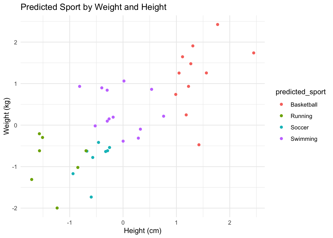
Now, I’ll create a KNN analysis on that data:
# Split data into training and testing setsset.seed(123)training_index <-createDataPartition(athletes_data$sport, p = .8, list =FALSE)training <- athletes_data[training_index, ]testing <- athletes_data[-training_index, ]# Normalise datapreproc <-preProcess(training[, -1])training_norm <-predict(preproc, training)testing_norm <-predict(preproc, testing)# Train KNN modelset.seed(123)knn_model <-knn(train = training_norm[, -1], test = testing_norm[, -1], cl = training_norm$sport, k =5)# Visualise classificationtesting_norm$predicted_sport <- knn_modelggplot(testing_norm, aes(x = height, y = weight, color = predicted_sport)) +geom_point() +labs(title ="Predicted Sport by Weight and Height", x ="Height (cm)", y ="Weight (kg)") +theme_minimal()
## ---------------------------## look at some model metrics# Actual vs. Predictedactual_sports <- testing_norm$sportpredicted_sports <- knn_model# Confusion Matrixconfusion_matrix <-table(Predicted = predicted_sports, Actual = actual_sports)print("Confusion Matrix:")
# Install and load caret if not already installed/loaded for additional metricslibrary(caret)# Other performance metricsperformance_metrics <-confusionMatrix(data =as.factor(predicted_sports), reference =as.factor(actual_sports))print(performance_metrics)
Confusion Matrix and Statistics

            Reference
Prediction   Basketball Running Soccer Swimming
  Basketball          9       0      0        2
  Running             0       5      2        0
  Soccer              0       3      4        1
  Swimming            0       0      5        8

Overall Statistics

               Accuracy : 0.6667
                 95% CI : (0.4978, 0.8091)
    No Information Rate : 0.2821
    P-Value [Acc > NIR] : 6.856e-07

                  Kappa : 0.5533

 Mcnemar's Test P-Value : NA

Statistics by Class:

                     Class: Basketball Class: Running Class: Soccer
Sensitivity                     1.0000         0.6250        0.3636
Specificity                     0.9333         0.9355        0.8571
Pos Pred Value                  0.8182         0.7143        0.5000
Neg Pred Value                  1.0000         0.9063        0.7742
Prevalence                      0.2308         0.2051        0.2821
Detection Rate                  0.2308         0.1282        0.1026
Detection Prevalence            0.2821         0.1795        0.2051
Balanced Accuracy               0.9667         0.7802        0.6104
                     Class: Swimming
Sensitivity                   0.7273
Specificity                   0.8214
Pos Pred Value                0.6154
Neg Pred Value                0.8846
Prevalence                    0.2821
Detection Rate                0.2051
Detection Prevalence          0.3333
Balanced Accuracy             0.7744
73.5 Decision trees
Theory
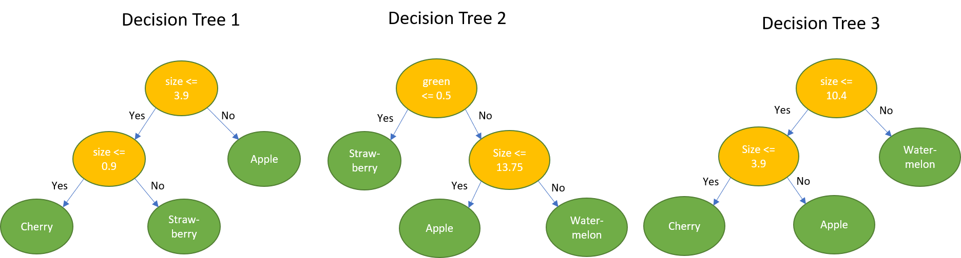
Decision Trees are a type of supervised learning algorithm that can be used for both classification and regression tasks. They’re intuitive and easy to understand, making them a popular choice in machine learning.
A decision tree splits the data into subsets based on the value of input features. This process is repeated recursively, resulting in a tree-like model of decisions.
In the context of machine learning, decision trees are built using algorithms that determine how to split the data best to maximize the homogeneity of the resultant nodes or minimize impurity (such as Gini impurity or entropy). The end nodes (or leaf nodes) of the tree represent the output predictions based on the input features traversed from the root to the leaf.
Example
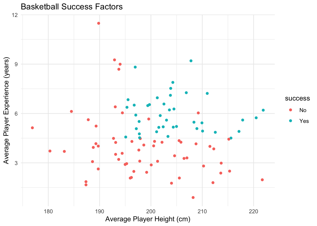
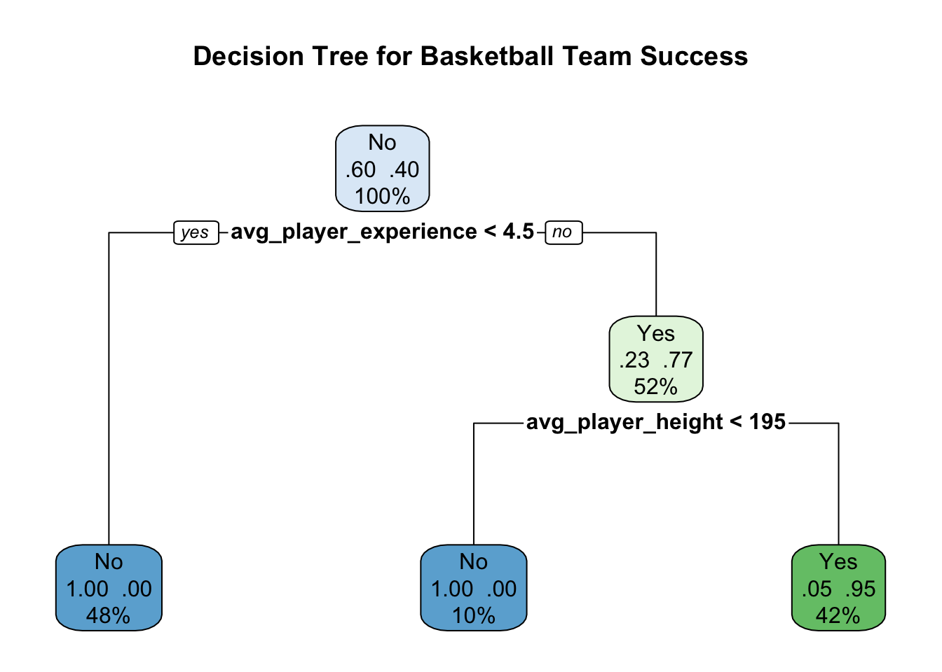
My task is to create a decision tree to determine the factors influencing the success of a basketball team.
First, I’ll create a dataset and perform an initial visualisation:
Code
library(tidyverse)
── Attaching core tidyverse packages ──────────────────────── tidyverse 2.0.0 ──
✔ dplyr     1.1.4     ✔ readr     2.1.5
✔ forcats   1.0.0     ✔ stringr   1.5.1
✔ lubridate 1.9.3     ✔ tibble    3.2.1
✔ purrr     1.0.2     ✔ tidyr     1.3.0
── Conflicts ────────────────────────────────────────── tidyverse_conflicts() ──
✖ dplyr::filter() masks stats::filter()
✖ dplyr::lag()    masks stats::lag()
✖ purrr::lift()   masks caret::lift()
ℹ Use the conflicted package (<http://conflicted.r-lib.org/>) to force all conflicts to become errors
Code
set.seed(123)# Generate datanum_teams <-100avg_player_height <-rnorm(num_teams, mean =200, sd =10)avg_player_experience <-rnorm(num_teams, mean =5, sd =2)games_won <-rpois(num_teams, lambda =30)success <-as.factor(ifelse(avg_player_height >195& games_won >20& avg_player_experience >4.5, "Yes", "No"))# Combine into a dataframetrain_data <-data.frame(success, avg_player_height, avg_player_experience, games_won)# Visualise dataggplot(train_data, aes(x = avg_player_height, y = avg_player_experience, color = success)) +geom_point() +labs(title ="Basketball Success Factors",x ="Average Player Height (cm)",y ="Average Player Experience (years)") +theme_minimal()
Now, I’ll run a decision tree analysis on that data, to analyse and predict the success of teams based on predictive factors:
# Load librarieslibrary(rpart)library(rpart.plot)# Create modeltree_model <-rpart(success ~ avg_player_height + avg_player_experience + games_won,data = train_data, method ="class")# Assuming avg_player_height and avg_player_experience are your intended variables and they are correctly named in train_datatree_model <-rpart(success ~ avg_player_height + avg_player_experience + games_won,data = train_data, method ="class")# Visualize the decision treerpart.plot(tree_model, main ="Decision Tree for Basketball Team Success", extra =104)
73.6 Neural networks
Theory
Neural networks are a set of algorithms designed to recognisepatterns. They interpret sensory data through a kind of machine perception, labeling, or clustering of raw input.
These algorithms loosely mimic the way a human brain operates, with neuron nodes interconnected like a web. While traditional algorithms build analysis with data in a linear way, neural networks process data in a non-linear approach.
Neural networks have a few important features:
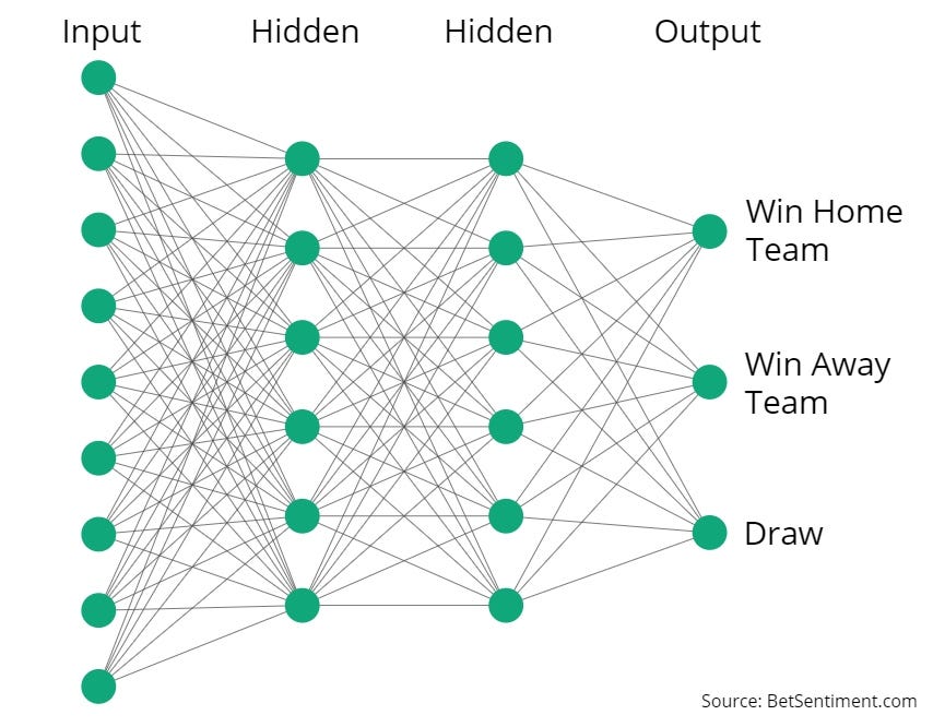
An Input Layer: This is where the network receives the data. Each node represents one feature of your data, like GDP per capita or population in our Olympic medals example below. Think of these nodes as the starting point for the data’s journey through the network.
Hidden Layers and Neurons: After the input layer, the data moves to hidden layers. These layers are where the neural network starts to understand and process the information. Each neuron in these layers performs calculations on the incoming data, transforming it step by step. The number of hidden layers and neurons can vary, but each one contributes to the network’s ability to learn from data.
Weights: Connections between neurons have associated weights. These weights determine the strength and direction (positive or negative influence) of the connection between neurons. During training, the network adjusts these weights to reduce errors in its predictions.
Activation Functions: Neurons use these mathematical functions to decide how much signal to pass forward. They help the network introduce non-linearities, enabling it to learn complex patterns.
Output Layer: This is the final stage of the network where it produces the result. In the example below, the output would be the predicted number of Olympic medals. The way data has been transformed and combined across layers culminates in this predicted value.
Training the Network: Training involves feeding the network data for which we know the outcome, allowing it to adjust its weights to make better predictions. Over time, the network learns from its mistakes, improving its accuracy.
Interpreting Results: After training, you can use the network to make predictions. By feeding in new input data, you can observe the output the network produces. The performance of the network can be evaluated by comparing its predictions to known outcomes.
Think of a neural network like a team playing through a season. The hidden layers are like the training sessions between games where the team (data) gets better and learns new strategies (features).
Initially, your team learns basic skills (simple patterns in data) in early training sessions (first hidden layers). As the season progresses, training gets more advanced (layers capture more complex patterns). Each session builds on the last, refining the team’s skills and strategies so they can tackle tougher opponents (make more accurate predictions or decisions).
By the end of the season (final layer), your team has gone through many levels of training (hidden layers), each more advanced than the last, preparing them to win the final game (make a final, accurate decision based on all they’ve learned).
Example (1)
I’m going to start with a very simple network.
We have a dataset of 10 countries. We are trying to predict the number of medals each country is likely to win, based on some predictors that we know such as GDP, population, and average training hours of their athletes,
library(neuralnet)
Attaching package: 'neuralnet'
The following object is masked from 'package:dplyr':

    compute
set.seed(123)# Creating synthetic datasetnum_countries <-10GDP_per_capita <-runif(num_countries, 1000, 50000) population_millions <-runif(num_countries, 1, 50)avg_training_hours <-runif(num_countries, 10, 15)medals_won <-round(0.001* GDP_per_capita +0.02* population_millions +0.5* avg_training_hours +rnorm(num_countries, 0, 2))olympic_data <-data.frame(GDP_per_capita, population_millions, avg_training_hours, medals_won)# Normalise data for performancemaxs <-apply(olympic_data, 2, max)mins <-apply(olympic_data, 2, min)scaled_olympic_data <-as.data.frame(scale(olympic_data, center = mins, scale = maxs - mins))# Define and train simple neural network with one hidden layer with two neuronsset.seed(123)nn_model <-neuralnet(medals_won ~ GDP_per_capita + population_millions + avg_training_hours, data = scaled_olympic_data, hidden =2, # Two neurons in the hidden layerlinear.output =TRUE,threshold =0.01)# Visualise neural networkplot(nn_model)
Each connection’s weight indicates the influence of one neuron’s output on the next neuron’s activation.
This visualisation helps us grasp how the inputs are being transformed through the network to arrive at the medal count prediction.
Example (2)
I’m going to expand that network to include more countries. Again, we’re trying to create a neural network to forecast the number of medals a country will win in the Olympics.
The plotted neural network provides insights into the learnedweights and structure.
Each neuron in the hidden layers extracts features from the input data, and the final layer combines these to forecast the number of medals won.
You can use the trained network to predict the medal count for new data, which might help us to understand the potential impact of different performance metrics on Olympic success.
73.7 Support Vector Machines
Theory
Support Vector Machines (SVM) are a set of supervised learning methods used for classification, regression, and outlier detection.
Imagine your’re the coach, and your team is preparing for an important match. To win, you need to find the best strategy to separate your team’s style of play from the opponent’s. You want to make sure your strengths are maximised and their weaknesses are exploited.
Support Vector Machines (SVM) work somewhat similarly in data classification. Think of SVM as a strategy to find the best possible line (or ‘hyperplane’ in more complex scenarios) that separates different categories of data. It’s like finding the optimal game plan that clearly distinguishes your team’s playing style from the opponent’s.
In SVM, the data points closest to the line from both teams are the key players (support vectors) because they help define the best separation strategy. The SVM focuses on maximising the margin between these key players and the line, ensuring that the strategy is as robust as possible.
So, just as your team would focus on a strategy that best leverages your strengths against the opponent’s weaknesses, SVM finds the best boundary that separates different categories, ensuring that new, unseen data (like a new game) can be accurately classified based on this optimal separation strategy.
Example
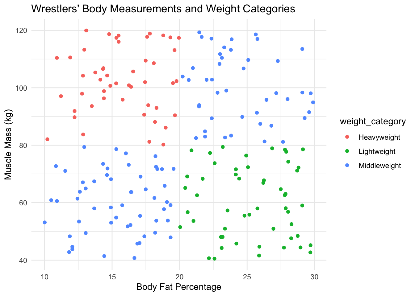
In this example, I’m going to use SVM to classify wrestlers into weight categories based on their body measurements.
# Load library# Load necessary librarylibrary(e1071)# Set seed for reproducibilityset.seed(123)# Generate synthetic data for wrestlersnum_wrestlers <-200body_fat_percentage <-runif(num_wrestlers, 10, 30) # Body fat percentagemuscle_mass_kg <-runif(num_wrestlers, 40, 120) # Muscle mass in kg# Define weight categories based on simple rules and random variation# Ensure weight_category is a factorweight_category <-factor(ifelse(body_fat_percentage <20& muscle_mass_kg >80, "Heavyweight",ifelse(body_fat_percentage >=20& muscle_mass_kg <=80, "Lightweight", "Middleweight")))wrestlers_data <-data.frame(body_fat_percentage, muscle_mass_kg, weight_category)# Check for NAs in your datasetsum(is.na(wrestlers_data))
[1] 0
# Visualize the datalibrary(ggplot2)ggplot(wrestlers_data, aes(x = body_fat_percentage, y = muscle_mass_kg, color = weight_category)) +geom_point() +labs(title ="Wrestlers' Body Measurements and Weight Categories", x ="Body Fat Percentage", y ="Muscle Mass (kg)") +theme_minimal()
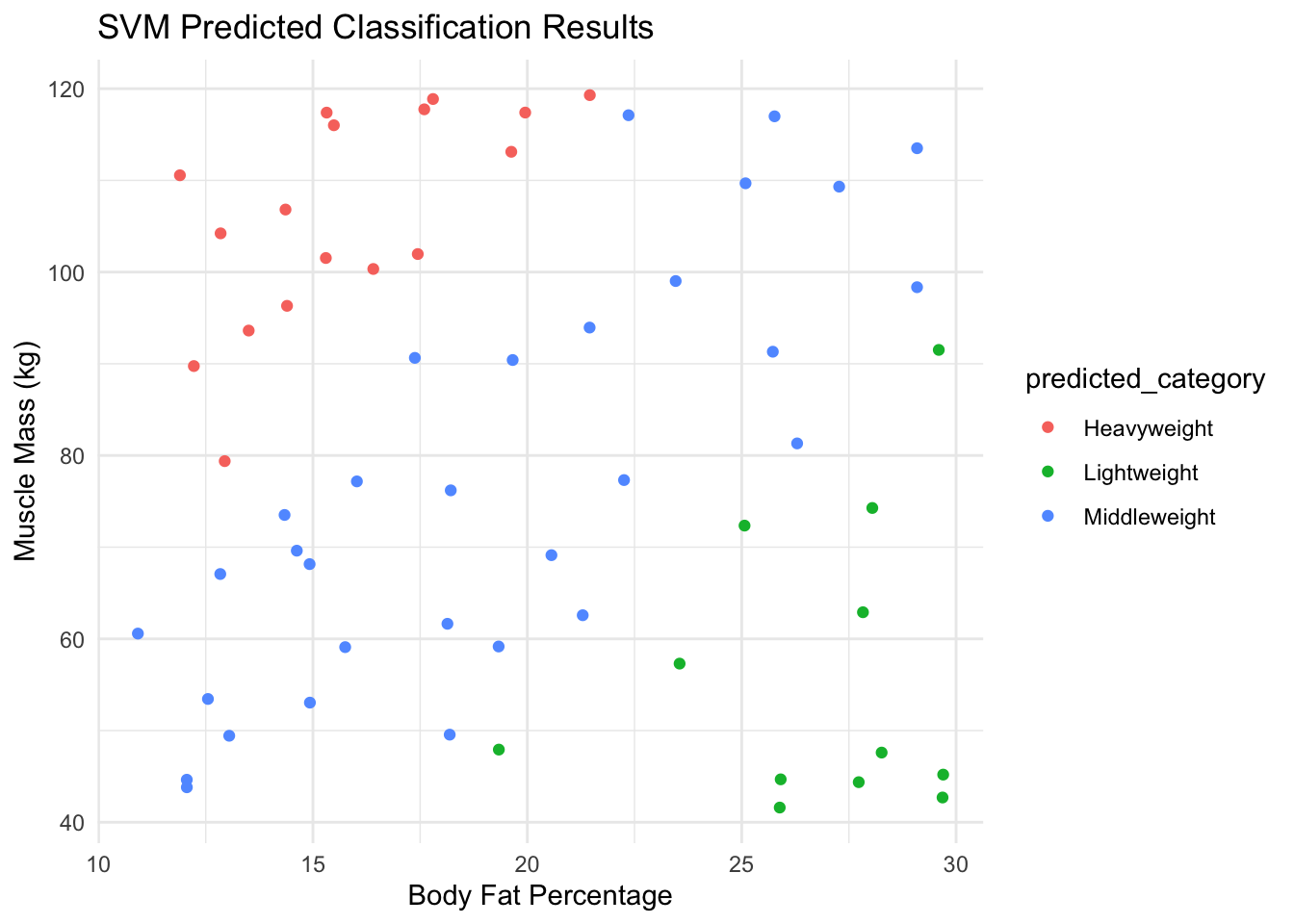
Now, I’m going to use SVM to try to categorise wrestlers appropriately.
# Splitting the dataset into training and testing setsindices <-sample(1:nrow(wrestlers_data), size =0.7*nrow(wrestlers_data))train_data <- wrestlers_data[indices, ]test_data <- wrestlers_data[-indices, ]# Train the SVM modelsvm_model <-svm(weight_category ~ ., data = train_data, type ='C-classification', kernel ='linear')# Predict using the SVM modelpredictions <-predict(svm_model, test_data)# Visualize the classification resultstest_data$predicted_category <- predictionsggplot(test_data, aes(x = body_fat_percentage, y = muscle_mass_kg, color = predicted_category)) +geom_point() +labs(title ="SVM Predicted Classification Results", x ="Body Fat Percentage", y ="Muscle Mass (kg)") +theme_minimal()
73.8 Conclusion
In this section, we’ve explored a variety of machine learning algorithms, each of which has its unique strengths and applications.
We began with regression: Regression algorithms are fundamental in predicting outcomes based on continuous data. For instance, in sport, regression can help predict the number of points a player might score in a game based on their past performance metrics. Remember that regression is a linear approach, assuming a direct relationship between input variables and the output.
We then moved on to logistic regression. Unlike linear regression, logistic regression is used for binary classification tasks. For example, it could classify whether a football team wins or loses based on certain match statistics. It provides probabilities for the outcome, giving us insight into the certainty of predictions made by the algorithm.
Both forms of regression were examples of supervised learning, where we give the model all the information we have and specify the IVs and DVs. We also learned about unsupervised models, where we don’t specify associations or outcomes.
K-Means Clustering is an example of an unsupervised learning algorithm, meaning it doesn’t require labelled data. In sport, k-means can group similar athletes together based on attributes like speed, strength, and endurance without prior knowledge of their categories. It ’s particularly useful in understanding player profiles, for example in the context of talent scouting.
Decision Trees, like K-means algorithms, are fairly intuitive and easy to understand. In sport, a decision tree could help determine the in-game playing strategy for a tennis player by considering various factors like opponent’s weakness, player’s stamina, and match conditions. It creates a tree-like model of decisions and their possible consequences, helping us select the most appropriate pathway.
We finished with two more complex algorithms, starting with Neural Networks. Mimicking the human brain’s structure, neural networks are powerful for capturing complex patterns. They could, for example, forecast a team’s season performance by learning from a vast array of historical data, including player statistics, weather conditions, and more. Neural networks excel in environments where relationships between variables are intricate and non-linear.
Finally, we examined Support Vector Machines (SVM): SVM is particularly effective for classification and regression with clear margin separation. In a sport context, SVM could categorise players into categories based (for example) on their physical measurements. SVMs are good at optimising the margin between different groups for robust classification.
All these algorithms aim to either make predictions or categorise data based on input features.
As such, they can be usefully applied to various sport analytics tasks, from performance prediction to strategic planning and player classification.
All of the algorithms rely on data to learn patterns, whether supervised (with labeled outcomes) or unsupervised (without labeled outcomes).
There are some important differences between the algorithms which we should bear in mind when deciding which approach to take.
In terms of supervision, regression, logistic regression, decision trees, neural networks, and SVM are supervised learning algorithms, requiring labelled data. In contrast, k-means is unsupervised.
In terms of the output type they can handle, regression predicts continuous outcomes, logistic regression handles binary outcomes, and neural networks and SVM can tackle both depending on their configuration. Decision trees and k-means are more categorically oriented.
In terms of their complexity and interpretability, I would suggest that decision trees are among the most interpretable models, while neural networks are more like “black boxes.” SVM and regression models offer a balance, depending on their kernel or complexity.
In terms of data structure, neural networks are suited for complex data with intricate patterns, while k-means and decision trees are best at handling simpler, categorical data. Regression models require numerical input features, which might not always be available to you.